Curve fitting by the method of least squares: fitting the lines y= a + bx and x = a + by

• Curve fitting is a statistical technique used to determine the best-fitting curve for a given set of data points.

• In the method of least squares, the goal is to minimize the sum of the squares of the differences between the observed values and the values predicted by the model.

Two common linear models are:

1. y = a + bx:

• This is the standard linear regression model where we predict the dependent variable y based on the independent variable xxx.

2. x = a + by:

• This is an alternate form where we predict xxx based on y.

Pharmaceutical Example

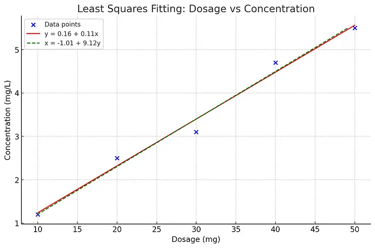
• Let's consider a pharmaceutical example where we are studying the relationship between the dosage of a drug (mg) and the resulting concentration of the drug in the blood (mg/L) after a certain period.

Example Data

Least Squares Fitting

1. Fitting y = a + bx:

• We fit a line to predict the concentration y based on the dosage xxx.

2. Fitting x = a + by:

• We fit a line to predict the dosage xxx based on the concentration y.

Let's perform the curve fitting and visualize the data.

Fit the line y = a + bx using least squares method.

Fitting x = a + by:

Let's perform these calculations and plot the data along with the fitted lines.

Analysis and Graph

Fitted Equations

• For y = a + bx

  • y = −0.96 + 0.112x

• For x = a + by

  • x = −1.01 + 9.12y

Explanation

In the context of our pharmaceutical example:

1. Y = a + bx: This model predicts the blood concentration of the drug (y) based on the dosage (x). The positive slope (b ≈ 0.112) indicates that as the dosage increases, the concentration in the blood increases.

2. X = a + by: This alternate model predicts the dosage (xxx) based on the blood concentration (y). The high slope (b ≈ 9.12) suggests that a small change in concentration requires a significant change in dosage.

Table Summary